Classification on EEG only datasets
In this post I will talk about the application of this package to classify EEG data. The purpose is to be able to classify an EEG alone, without an fMRI pairing, while being able to project a synthesized fMRI view.
EEG only dataset
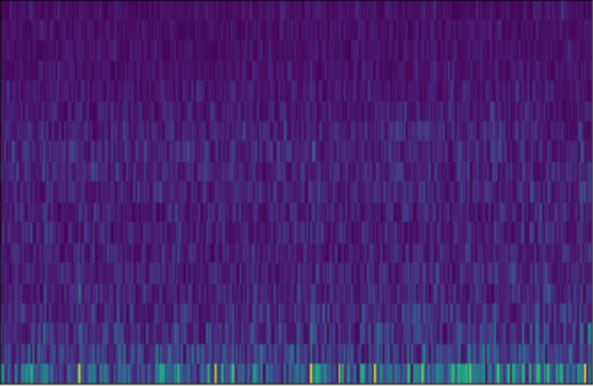
The dataset consists of \(N\) individuals. The individuals have a set of features \(X \in \mathbb{R}^{N \times C\times F\times T}\) and labels \(y \in \mathbb{R}^{N \times 1}\). The notation is similar to the previous blog post, where \(C\) stands for the number of channels, \(F\) is the frequency resolution and \(T\) is the amount of time considered of the EEG recording. An EEG instance looks like illustrated in the figure below.

This image corresponds to the STFT projection of one channel. The labels are \(y = \{0, 0, \dots, 1, 1\}\). Note that, we only consider binary classification problems for this setup.
Classifying synthesized images
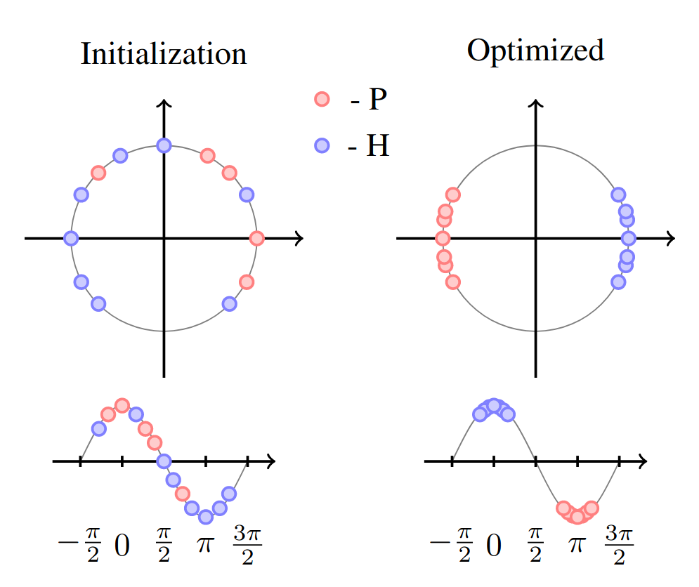
In this section, I will go over the methodology used to classify synthesized images (projected by sinusoids). This is the novel contribution of this paper. Let \(\vec{z}_{X_i}=E(X_i; \theta_E)\) be a latent projection of the synthesizer model preceding the sinusoid projection. Since the sinusoid projection is \(cos(\omega \cdot \vec{z}_{X_i} + \beta)\), with \(\omega,\beta\) being trainable parameters, then we can by induction separate both \(\omega \cdot \vec{z}_{X_i} + \beta\) and \(cos(\omega \cdot \vec{z}_{X_i} + \beta)\) using a contrastive loss. In the figure below it is shown how the points are initialized and how after training they are well separated in opposite sides of the unit circle, where the \(cos\) takes values \(\approx 1\) and \(\approx -1\).

The loss that achieves this goal is an adaptation of the contrastive loss [1],
\[\mathcal{L}_D(X_1, X_2, y_p) = y_p \times D(X_1, X_2) + (1-y_p) \times \|D(X_1,X_2)-m\|_1,\]where \(X_1\) and \(X_2\) are the two instances that constitute the pair. The distance function is defined as \(D(X_i, X_j)=\|(\omega \cdot\vec{z}_{X_i} + \beta) -(\omega \cdot \vec{z}_{X_j} + \beta)\|_1\) and \(y_p\) specifies if these two instances belong together or not. Two instances belong together if \(y_i == y_j\) and are false pairs if \(y_i \neq y_j\). Therefore, \(y_p\) can be represented as \(1[y_i == y_j]\). The term \(y_p \times D(X_1, X_2)\) brings points with the same label closer together, while them term \((1-y_p) \times \|D(X_1,X_2)-m\|_1\) places points with different labels as far as \(m\), which we set to \(m=\pi\).
Let us dive into the code!
First you need to do all the imports:
import tensorflow as tf
from utils import data_utils, preprocess_data, tf_config, train, losses_utils, lrp, viz_utils, fmri_utils
from models import classifiers, eeg_to_fmri
from pathlib import Path
import numpy as np
import matplotlib.pyplot as plt
from pathlib import Path
import pickle
Then you set up the information about which dataset to use for the classification, for the synthesis, as well as setting up the seed for tensorflow and the memory limit it uses on the GPU.
dataset="11"
dataset_synthesis="01"
raw_eeg=False
n_individuals=getattr(data_utils, "n_individuals_"+dataset)
memory_limit=1500
interval_eeg=10
tf_config.set_seed(seed=2)
tf_config.setup_tensorflow(device="GPU", memory_limit=memory_limit, run_eagerly=True)
For this classification setting, we always assume a CV with \(5\) folds, but here we simply do one fold. That is why the number of folds is being set, but only one of them is being considered train_data, test_data = dataset_clf_wrapper.split(0).
with tf.device('/CPU:0'):
	dataset_clf_wrapper = preprocess_data.Dataset_CLF_CV(dataset, standardize_eeg=True, load=True)
	dataset_clf_wrapper.shuffle()
	dataset_clf_wrapper.set_folds(5)
	train_data, test_data = dataset_clf_wrapper.split(0)
	X_train, y_train=train_data
	X_test, y_test=test_data
With the train and test data, which formulate the pairs of data \(X, y\), with its corresponding features and labels we are set. Wait! We still need a special type of pairing for the training, since we are minimizing the contrastive loss. That means we need pairs of instances \(i, j\), where for each batch introduced in the model we need their features \(X_i, X_j\), labels \(y_i, y_j\) and pair label \(y_p = 1[y_i==y_j]\). In the end each batch of the train_set contains tuples of the form \((X_i, X_j, y_p, y_i, y_j)\).
train_set = preprocess_data.DatasetContrastive(X_train, y_train, batch=8, clf=True)
test_set = tf.data.Dataset.from_tensor_slices((X_test, y_test)).batch(1)
Why do we need the labels \(y_i, y_j\)? Because in addition to separating the data according to the contrastive loss, we are also learning a linear classifier that classifies the synthesized fMRI view. This loss is represented as
\[\mathcal{L}_C(X_i, X_j, y_i, y_j) = y_i\times log(\hat{y}_i) + y_j\times log(\hat{y}_j),\]where both instances are used for the training of the classifier. Please note that \(\hat{y}=f(X)\) is the label prediction of the whole function, that in between synthesizes an fMRI volume. Altogether, these losses form the main loss
\[\mathcal{L}(X_i, X_j, y_p, y_i, y_j) = \mathcal{L}_D(X_i, X_j, y_p) + \mathcal{L}_C(X_i, X_j, y_i, y_j) + \lambda\|\theta\|_1,\]where \(\theta\) is the set of parameters of the classifier only. This loss is built in the losses_utils module and is instantiated in the code as:
loss_fn=losses_utils.ContrastiveClassificationLoss(m=np.pi, reduction=tf.keras.losses.Reduction.SUM_OVER_BATCH_SIZE)
Please check the Linear Classifier and Dense Variational modules to see the code used to classify a synthesized fMRI view (of the EEG).
Now that we have all the data setted up, we can start building the model.
network="/home/ist_davidcalhas/eeg_to_fmri/networks/deterministic"
optimizer = tf.keras.optimizers.Adam(1e-3)
linearCLF=classifiers.ViewLatentContrastiveClassifier(tf.keras.models.load_model(network,custom_objects=eeg_to_fmri.custom_objects), X_train.shape[1:], activation=tf.keras.activations.linear, regularizer=tf.keras.regularizers.L1(l=2.), variational=True)
linearCLF.build(X_train.shape)
With the model built, we only have the training session left to do:
train.train(train_set, linearCLF, optimizer, loss_fn, epochs=10, verbose=True, verbose_batch=True)
The output corresponds to:
<<< Epoch 1 with loss: 84.25851927132442
<<< Epoch 2 with loss: 52.9350555025298
<<< Epoch 3 with loss: 125.1430987325208
<<< Epoch 4 with loss: 78.96974868609988
<<< Epoch 5 with loss: 57.1884643990418
<<< Epoch 6 with loss: 60.4331891588096
<<< Epoch 7 with loss: 38.95034251619002
<<< Epoch 8 with loss: 10.687810596078634
<<< Epoch 9 with loss: 19.28891693029938
<<< Epoch 10 with loss: 6.3919262424882115
The training loss does not converge in the beginning, which is due to the loss being composed by two components that are dependent. For the classification loss to converge, the contrastive loss needs to converge in the first place. This is why the values of the training loss do not look very stable. However, the model is still learning the tasks defined, let’s see what it synthesizes and how it performs predictively.
for x, _ in test_set.repeat(1):
	fig = viz_utils.plot_3D_representation_projected_slices(linearCLF.view.q_decoder(x).numpy()[0,:,:,:,:],slice_label=True, threshold=0.50,)
	break
Now we can use the fMRI synthesized view to check which regions of the synthesized brain had more relevance to the prediction.
explainer = lrp.LRP(linearCLF.clf)
test_views = np.empty((0,)+getattr(fmri_utils, "fmri_shape_"+dataset_synthesis)+(1,))
for x, _ in test_set.repeat(1):
    test_views = np.append(test_views, linearCLF.view.q_decoder(x), axis=0)
test_views_set = tf.data.Dataset.from_tensor_slices((test_views,y_test)).batch(1)
R=lrp.explain(explainer, test_views_set, verbose=True)
fig = viz_utils.plot_3D_representation_projected_slices(np.mean(R, axis=0), res_img=np.mean(fmri_train,axis=0),slice_label=True,cmap=plt.cm.gist_heat,threshold=0.2,legend_colorbar=r"$\mathbb{E}[R]$",max_min_legend=["Negative","Positive"])